
Overview
When negotiating the sale of a business, contingent consideration provisions are oftentimes incorporated as a component of the total purchase price to close the disparity between the buyer’s and the seller’s expectations regarding the target company value. Additionally, contingent consideration provisions allow buyers and sellers to: (1) defer a portion of the purchase consideration to a later date, (2) incentivize and motivate sellers post-transaction, (3) provide a mechanism to allocate a portion of a transaction’s risk and reward from the buyer back to the seller, and (4) offset a portion of the buyers’ (equity and debt) capital needed at closing. Buyers may be more willing to pay a higher total price for a business if the seller is willing to make a portion of the value contingent on the target company’s ability to achieve certain milestones post-acquisition. At the same time, the seller may be more willing to accept a lower base price if they are confident that the company can achieve certain performance goals, thereby realizing the contingent consideration and higher total price.
Contingent consideration may represent either an obligation for the acquirer to transfer additional cash, other assets or equity interests to the former owner (an “earn-out”) or an acquirer’s right to recapture previously transferred (typically) non-cash consideration, i.e. seller notes (a “clawback”), if pre-specified events occur or, alternatively, if certain results are not achieved in the future. From the acquirer’s perspective, an earn-out may be accounted for as a liability, while a clawback may be accounted for as an asset. However, for valuation purposes, whether the contingent consideration represents an earn-out or a clawback, it is appropriate to frame the valuation of contingent consideration as the valuation of an asset. Whether the contingent consideration represents an earn-out or a clawback, each form carries with them unique tax considerations outside the scope of this white paper.
The consideration itself may take the form of cash payments, additional shares in the acquirer or an enhanced return prerogative, similar to a 1.5x or 2.0x preferred return in a security received in exchange. For discussion purposes, the balance of this white paper addresses contingent consideration in the form of cash payment(s). However, if there are enhanced rollover equity proceeds, the valuation of those securities ought to be considered in conjunction with the uncertainty of achieving the contingent component of the contingent consideration.
Contingent Consideration Characteristics
Each contingent consideration contains characteristics specific to its purpose and the operations of the subject company. Contingent consideration may be based on outcomes or events specific to a company’s customer relationships or its ability to successfully develop products or technology. In this case, the payoff is often structured in an all-or-nothing manner, in which the outcome determines whether the contingent consideration is paid. Alternatively, contingent consideration may be based on a company’s relative performance and measured by revenue, earnings or output, measured in units.
Contingent consideration related to events and performance may be measured by financial metrics or non-financial events. Examples of financial and non-financial metrics include:
Financial Metrics: Revenue, EBITDA, net income and business metrics such as number of units sold.
Non-Financial Milestone Events: Regulatory approvals, success or retention of specific contracts with customers or the achievement of a product launch or stage of product development.
The risk associated with an underlying metric affects the required return, or discount rate, relied upon to estimate the fair value of a contingent consideration. The type of risk associated with an underlying metric may be broadly categorized as either diversifiable or non-diversifiable depending on the metric’s relationship, or correlation, with the broader markets. Generally, market participants reduce risk through diversification and will only require a return premium above the risk-free rate for risk that cannot be diversified away.
In the context of contingent consideration, the risk associated with non-financial metrics is considered diversifiable, since their respective outcomes are not typically influenced by movements in the market. For example, the likelihood of a pharmaceutical drug receiving approval and advancing to the next stage of development is not necessarily affected by market performance; therefore, outcome’s risk is considered diversifiable. If the risk associated with the underlying metric is diversifiable, then the discount rate applied to the cash flow contingent on the metric is based on a risk-free rate plus an adjustment for counter-party credit risk, if applicable. On the other hand, the risk associated with a financial metric is not fully diversifiable. Therefore, market participants require a risk premium above the risk-free rate as compensation for the non-diversifiable risk.
Contingent Consideration Structures
The structure of a contingent consideration determines the relationship between the performance (or outcome) of an underlying metric and its resulting payoff. A contingent consideration payoff may be structured as either a fixed payment or a fixed percentage of the underlying metric; thus, its structure may be defined as either linear or non-linear depending on the existence of certain complexities such as thresholds, caps or tiers.
For a non-financial metric with diversifiable risk, the payoff structure does not affect the magnitude of the required rate of return. However, if the underlying metric is a financial metric with non-diversifiable risk, the payoff structure may affect the overall risk of the earn-out. The difference between the risk associated with the earn-out and the risk associated with the underlying financial metric is dependent upon whether the payoff structure is linear or non-linear. For a financial metric with a non-linear payoff structure, the risk of the payoff will depend on the risk associated with the metric and the probability of achieving a certain contingency. Therefore, the larger the degree of risk associated with a particular payoff structure, the larger the difference may be between the risk of the underlying metric and the risk of the contingent consideration payoff.
The relationship between the payoff structure and the performance of an underlying financial metric for various structures is illustrated below:
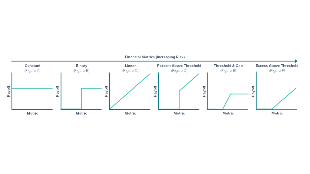
A constant payoff structure (Figure A) represents a fixed yet deferred payoff, regardless of the underlying metric’s performance. Conversely, a binary payoff structure (Figure B) represents a payoff where the amount of payoff is fixed but dependent on the underlying metric meeting or exceeding a pre-specified threshold level. The existence of a threshold introduces an element of risk that is specific to a contingent consideration’s non-linear structure.
The introduction of contingencies such as thresholds and or caps may increase the risk associated with a particular contingent consideration. Additionally, the existence of multiple contingencies, such as the combination of a threshold and a cap (Figure D) or a payoff that is calculated as a percentage of excess above a threshold (Figure F), may introduce a greater degree of risk compared to that of a contingent consideration with a payoff dependent on a single contingency such as one threshold.
The payoff of a contingent consideration based on a financial metric with a non-linear structure has two sources of risk. First, the risk of the underlying financial metric itself, and second, the risk introduced by the non-linear structure of the payoff, given that there is less than a 100% probability of achieving specified contingencies. The degree of risk introduced by a contingent consideration’s structure depends on the proximity of the expected metric forecast relative to various structural features, the expected volatility in growth for the metric and the time remaining to settlement. However, a payoff’s risk is not affected by whether the payoff structure is linear or non-linear when the contingent consideration is based on a non-financial metric with diversifiable risk.
A linear payoff structure (Figure C) represents a payoff structure where the contingent consideration pays a fixed percentage of a financial metric, such as revenue or EBITDA, and where there is a direct relationship between the payoff and the underlying metric’s performance. In this case, the risk associated with the metric is equivalent to the risk associated with the payoff.
Approaches to Contingent Consideration Valuation
The three generally-accepted valuation approaches to estimate the value of an asset or liability include the income approach, the market approach and the cost approach. Of the three approaches, the income approach is typically relied on to value contingent consideration. Within the income approach, there are two commonly-used methods to value contingent consideration.
- The scenario-based method (“SBM”)
- The option pricing method (“OPM”)
Although neither of the methods is considered to be universally superior to the other, each method has strengths and weaknesses that make it more or less appropriate depending on the characteristics of a particular contingent consideration.
Selecting a Valuation Methodology
Using the income approach, two methods commonly relied on to value a contingent consideration include the scenario-based method (“SBM”) and the option pricing method (“OPM”). Two key differences between the SBM and the OPM include:
The method’s ability to account for both the risk associated with the underlying metric and, if applicable, the risk associated with the contingent consideration’s payoff structure; and
The complexity associated with the process, including its required inputs and subsequent output
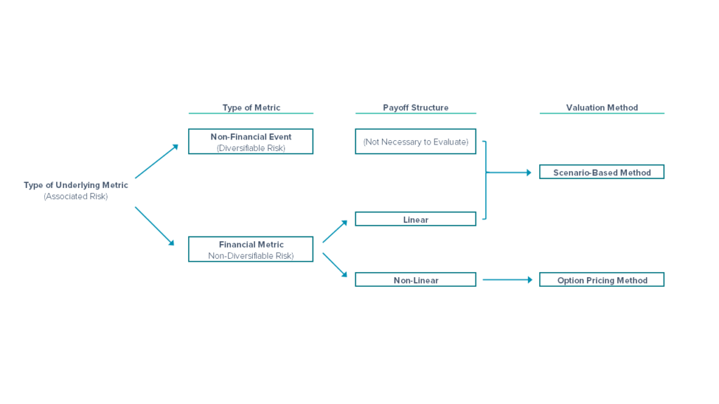
In selecting a method to determine the value of a contingent consideration, the first step is to identify the type of underlying metric upon which the payoff is dependent. If the underlying metric is a financial metric with non-diversifiable risk, the second step is to understand and categorize the structure of the payoff as either linear or non-linear. If the underlying metric is a non-financial metric, the payoff structure would not impact the decision between valuation methods.
The process of selecting the appropriate valuation method for a particular contingent consideration follows a decision tree based on their key differences, depicted on the next page.
The Scenario-Based Method (“SBM”)
The scenario-based method requires the identification of a set of outcomes (or scenarios) for the underlying metric or event and the payoffs associated with each outcome. The payoffs are then probability-weighted according to an assessment of the likelihood of each scenario. The probability-weighted payoffs are then discounted at the appropriate rate to calculate the expected present value of the contingent consideration.
The SBM is an appropriate method to use either when the risk of the underlying metric is diversifiable (a non-financial metric), or when the payoff structure is linear. While the process of calculating probability-weighted payoffs is similar regardless of whether the risk of the underlying metric is diversifiable or non-diversifiable, the discount applied to the probability-weighted payoff will depend on the underlying metric’s type of risk.
- If the risk of the underlying metric is event-based with diversifiable risk, the discount rate should account for the time value of money (risk-free rate) over the relevant time horizon and, if applicable, a premium for counterparty credit risk.
- If the risk of the underlying metric is a financial metric with non-diversifiable risk, the discount rate should account for the time value of money (risk-free rate) over the relevant time horizon, a premium for counterparty credit risk (if applicable) and a risk premium appropriate for the metric itself (the required metric risk premium or “RMRP”).
If the payoff structure is non-linear and the risk of the underlying metric is non-diversifiable, the discount rate should also account for risk attributable to the payoff structure itself. In order to accurately account for the payoff structure’s risk, the premium added to the discount rate would depend on the proximity of the expected metric value relative to the various structural features, the expected volatility for the metric’s growth rate and the time remaining to settlement. Due to the difficulty and complexity associated with such an estimation, the SBM is generally not utilized to estimate the value of a contingent consideration based on an underlying metric with non-diversifiable risk and a non-linear payoff structure.
The Option Pricing Method (“OPM”)
The option pricing method is commonly relied upon to value contingent consideration in which the underlying metric is a financial metric with non-diversifiable risk and the payoff structure is non-linear. The primary advantage of the OPM is that it circumvents the difficulties associated with estimating a discount rate to account for a particular payoff structure’s risk. Instead of estimating a discount rate that accounts for the risk of the underlying metric as well as the risk associated with the contingent consideration’s payoff structure, the OPM relies upon a risk-neutral framework in which the forecasted metric and expected payoff are separately discounted in two steps to account for the impact of a non-linear payoff structure on risk-adjusted cash flows.
First, the forecasted underlying metric is risk-adjusted by discounting the forecasted value by the appropriate RMRP to account for the underlying metric’s non-diversifiable risk. Since the underlying metric is exposed to non-diversifiable (or systematic) risk over the period during which it is earned, the forecasted metric is discounted by the RMRP using mid-period discounting convention. The risk-neutral forecast is then relied upon as an input for a closed-form solution or simulation (such as a Monte Carlo simulation) depending on the payoff function to calculate the expected payoff. Second, the expected payoff is then discounted to account for the time value of money and a premium for counterparty credit risk (if applicable) over the time horizon from expected payment date(s) to the transaction’s close date.
The OPM assumes that the expected value of the underlying metric is lognormally distributed and that the forecasted underlying metric follows a geometric Brownian motion (“GBM”). GBM is a statistical process in which the risk-adjusted metric is forecasted as a function of the logarithm of the expected growth rate plus a drift term. GBM provides a framework to account for various paths an underlying metric may take as it evolves over time, assuming the expected growth rate is independent and normally distributed. Additionally, GBM provides what may be considered a constraint on the growth rate for period-over-period values by implying continuity in the underlying metric. However, continuity does not mean the underlying metric will increase smoothly at a constant logarithmic growth rate. Rather, GBM reflects a statistically random component that is determined by the underlying metric’s volatility.
Key inputs for the OPM include:
- A forecasted expected (mean) value for the underlying metric over the relevant measurement period of the contingent consideration.
- An estimate of expected volatility of the underlying metric that is relevant to the time horizon from the transaction close date to the end of the metric’s measurement period.
- Discount periods relevant for both the period of time between the transaction close date and the end of the metric’s measurement period and the transaction close date to the estimated payment date.
- Discount rates to account for the risk of the underlying metric (RMRP), counterparty credit risk (if applicable) and the time value of money (risk-free rate).
Estimating the Required Metric Risk Premium (“RMRP”)
The required metric risk premium (RMRP) represents the return required to compensate market participants for the non-diversifiable risk associated with an underlying financial metric. In situations where the metric is not directly related to the value of the acquired company’s assets, the RMRP may be different from the company’s weighted average cost of capital (“WACC”) or the internal rate of return (“IRR”) indicated by the transaction price. Two methods commonly relied upon to estimate the RMRP include the top-down method and the bottom-up method.
The top-down method begins with the risk premium associated with the acquired company’s long-term free cash flow to the firm (“LTFCFF”) and adjusts the long-term risk premium for sources of risk that may or may not be applicable to the metric. For example, contingent consideration is generally based on the performance of an underlying metric over a short-term horizon, while the risk premium represented by the company’s WACC is long-term by nature. Accordingly, the components of the company’s WACC may be adjusted to reflect the appropriate time horizon for the underlying metric. Additionally, a company’s WACC accounts for risk attributable to the company’s capital structure and degree of financial leverage, whereas an earnings-based metric, such as EBIT, is not affected by financial leverage. Further, if the metric is a revenue-based metric, such as revenue or EBITDA, the company’s WACC should be adjusted to remove the degree of risk attributable to both financial leverage and operational leverage.
The bottom-up method estimates the metric’s risk premium with a direct estimate of the underlying metric’s beta to the broader market. Within the CAPM framework, additional risk premiums are then incorporated in the RMRP based on the portion of risk premiums included in the company’s WACC that are applicable to the underlying metric over the metric’s measurement period. Although estimating the metric’s beta requires historical data to calculate the metric’s volatility and correlation in growth relative to the market, the bottom-up method may circumvent the process of de-levering an estimated equity volatility for financial and operational leverage (if applicable).
Estimating Metric Volatility
In situations where a contingent consideration has a non-linear payoff structure, the expected volatility of the underlying metric’s forecasted growth affects the difference between the payoff calculated based on the metric’s forecasted value and the payoff calculated based on the risk-adjusted forecasted metric value. Generally, the payoff’s sensitivity to changes in estimated volatility will depend on where the base case forecast is relative to the earn-out thresholds and caps, as well as the time remaining from the transaction close date to the end of the metric’s measurement period.
The expected volatility for the underlying metric may be estimated based on the historical volatility of the underlying metric, management’s estimate of future outcomes for the metric or by de-levering the historical equity volatility of the acquired company. In situations where the acquired company is private, it may be appropriate to rely upon the historical equity volatility of guideline publicly-traded companies. The method relied upon to estimate the metric’s volatility may depend on the availability and reliability of the company’s historical financial data, the type of underlying metric and the similarity of identified guideline public companies, among other factors. For example, if the underlying metric is revenue-based, historical equity volatility may need to be adjusted, or de-levered, to account for both financial leverage and operational leverage, represented by the company’s forecasted fixed operating costs. If the company’s forecasted fixed costs are difficult to identify, but the company’s historical revenue is available and comparable (from an accounting or business segment perspective), it may be preferable to rely upon the historical volatility of the company’s revenue growth as an indication for the expected volatility.
Estimating Counterparty Credit Risk
Counterparty credit risk represents an additional premium to the time value of money (risk-free rate) to compensate for the default risk of the legal obligor (the buyer). Counterparty credit risk should account for the seniority of the contingent consideration in the acquirer’s capital structure, as well as the expected timing of the payment. The risk premium is typically the pre-tax cost of debt that aligns with the term and seniority of the obligation and should reflect buyer-specific credit risk.
Counterparty credit risk may be mitigated in some circumstances by terms within the contingent consideration, such as cash or collateral deposited in an escrow account, the seniority or securitization of the obligation or a guarantee from a bank or other party. Counterparty credit risk may also be mitigated if the acquired company is a large portion of the post-acquisition company, or when the acquired company and the buyer are affected by similar risk factors.
Monte Carlo Simulation
Contingent consideration structures that span multiple periods with path-dependent payoffs or structures that involve multiple, interdependent non-diversifiable metrics will generally require the use of a multi-variable technique such as Monte Carlo simulation. Monte Carlo simulation is a statistical process that simulates the outcome of a forecast over thousands of repeated trials. When key assumptions include growth rates and volatility, there may be a number of outcomes possible for a single forecast. Therefore, for a given forecast, the use of repeated trials may provide a significantly higher degree of confidence with a mean value compared to a single forecasted value.
In the context of contingent consideration, Monte Carlo simulation may be used to account for multiple time horizons or multiple interdependent underlying metrics by incorporating an assumed (joint) distribution for each metric, for each period. When there are multiple metrics, an estimate of the correlation between the metrics is required to determine the joint distribution. This may be estimated based on either the historical correlation between the metrics or an assessment of the relationship between the metrics provided by the company’s management.
After risk-adjusting the metrics’ forecast within the OPM’s risk-neutral framework, the payoff is calculated for each trial according to the contingent consideration’s structure. The payoff is then discounted from the expected payment date(s) to the transaction close date at the risk-free rate plus any adjustment for counterparty credit risk (if applicable). The value of the contingent consideration is then calculated as the mean present value of the payoffs across all of the simulation’s trials.
Conclusion
Each contingent consideration is characterized by terms and conditions unique to a specific transaction. From identifying and quantifying the sources of risk applicable to the contingent consideration, to selecting the appropriate inputs for valuation, contingent consideration can present a significant challenge to accounting teams, financial advisors and business owners alike. Whether you are evaluating a contingent consideration as part of the initial recognition and fair value measurement requirements under ASC 805, or contemplating the sale of a business to private equity groups, public companies or ESOPs, it’s important to fully understand the challenges associated with the valuation of contingent consideration. As such, consider partnering with a trusted and experienced advisor to help you navigate the contingent consideration valuation process.
Dan Callanan is a Managing Director at Prairie Capital Advisors, Inc. He can be contacted at 614.768.7301 or by email: dcallanan@prairiecap.com.
Rebecca McElwain is Director at Prairie Capital Advisors, Inc. She can be contacted at 614.768.7302 or by email: rmcelwain@prairiecap.com
Related Resources
View Allwebinar


